Excel VLOOKUP Tutorial for Beginners: Step-by-Step Examples

What is VLOOKUP?

VLOOKUP (V stands for ‘Vertical’) is an in-built function in excel which allows establishing a relationship between different columns of excel. In other words, it allows you to find (look up) a value from one column of data and returns it’s respective or corresponding value from another column.

In this VLOOKUP guide, we will learn

• Usage of VLOOKUP:
• How to use VLOOKUP function in Excel
• VLOOKUP for Approximate Matches (TRUE Keyword as the last parameter)
• VLOOKUP function applied between 2 different sheets placed in a same workbook

Usage of VLOOKUP:

When you need to find some information in a large data-spreadsheet, or you need to search for the same kind of information throughout the spreadsheet use the VLOOKUP function.

Let’s take an instance of VLOOKUP as:

Company Salary Table which is managed by the financial team of the Company – In Company Salary Table, you start with a piece of information which is already known (or easily retrieved). Information that serves as an index.

So as an Example:

You start with the information which is already available:

(In this Case, Employee’s Name)

To find the information you don’t know:

(In this case, we want to look up for Employee’s Salary)

Excel Spreadsheet for the above instance:

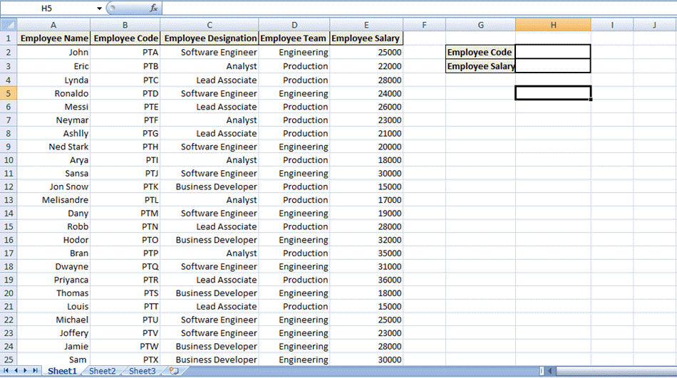
In the above spreadsheet, to find out the Employee Salary which we don know –

We will enter the Employee Code which is already available.

Moreover, By Applying VLOOKUP, value(Employee’s salary) of the corresponding Employee’s Code will be displayed.

How to use VLOOKUP function in Excel

Following is a step-by-step guide on how to apply the VLOOKUP function in Excel:

Step 1) Navigate to the cell where you want to view
We need to navigate to the cell where you want to view the Salary of the particular Employee.- (in this instance, Click the cell with index ‘H3’)

Step 2) Enter the VLOOKUP function =VLOOKUP ()
Enter the VLOOKUP Function in the above Cell: Start with an equal sign which denotes that a function is entered, ‘VLOOKUP’ keyword is used after the equal sign depicting VLOOKUP function =VLOOKUP ()

The parenthesis will contain the Set of Arguments (Arguments are the piece of data that function needs in order to execute).

VLOOKUP uses four arguments or pieces of data:

Step 3) First Argument – Enter the lookup value for which you want to look up or search.
The first argument would be the cell reference (as the placeholder) for the value that needs to be searched or the lookup value. Lookup value refers to the data which is already available or data which you know. (In this case, Employee Code is considered as the lookup value so that the first argument will be H2, i.e., the value which needs to be looked up or searched, will be present on the cell reference ‘H2’).

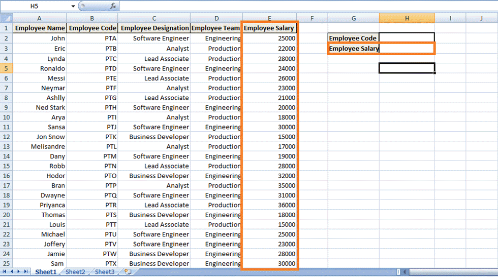
Step 4) Second Argument – The table array
It refers to the block of values that are needed to be searched. In Excel, this block of values is known as table array or the lookup table. In our instance, the lookup table would be from cell reference B2 to E25,i.e., the complete block where the corresponding value would be searched.

NOTE: The lookup values or the data you know have to be in the left-hand column of your lookup table,i.e., your cell range.

Step 5) Third Argument – VLOOKUP syntax is the column_index_no
It refers to the column reference. In other words, it notifies VLOOKUP where you expect to find the data, you want to view. (Column reference is the column index in the lookup table of the column where the corresponding value ought to be found.) In this case, the column reference would be 4 as the Employee’s Salary column has an index of 4 as per the lookup table.

Step 6) Fourth Argument – Exact match or approximate match
The last argument is range lookup. It tells the VLOOKUP function whether we want the approximate match or the exact match to the lookup value. In this case, we want the exact match (‘FALSE’ keyword).

1. FALSE: Refers to the Exact Match.
2. TRUE: Refers for Approximate Match.

1. 

Step 7) Press Enter!
Press ‘Enter’ to notify the cell that we have completed the function. However, you get an error message as below because no value has been entered in the cell H2i.e. No employee code has been entered in Employee Code which will allow the value for lookup.

However, as you enter any Employee Code in H2, it will return the corresponding value i.e. Employee’s Salary.

So in a brief what happened is I told the cell through the VLOOKUP formula is that the values which we know are present in the left-hand column of the data,i.e., depicting the column for Employee’s Code. Now you have to look through my lookup table or my range of cells and in the fourth column to the right of the table find the value on the same row,i.e., the corresponding value (Employee’s Salary) in the same row of the corresponding Employee’s Code.

The above instance explained about the Exact Matches in VLOOKUP., FALSE Keyword as the last parameter.

VLOOKUP for Approximate Matches (TRUE Keyword as the last parameter)

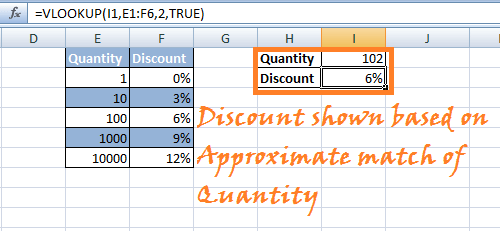
Consider a scenario where a table calculates discounts for the customers who do not want to buy exactly tens or hundreds of items.

As shown below, certain Company has imposed discounts on the quantity of items ranging from 1 to 10,000:

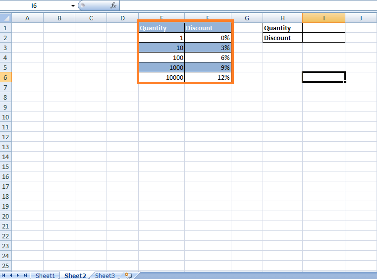
Now it is uncertain that the customer buys exactly hundreds or thousands of items. In this case, Discount will be applied as per the VLOOKUP’s Approximate Matches. In other words, we do not want to limit them for finding matches to just the values present in the column that are 1, 10, 100, 1000, 10000. Here are the steps:

Step 1) Click on the cell where the VLOOKUP function needs to be applied i.e. Cell reference ‘I2’.

Step 2) Enter ‘=VLOOKUP()’ in the cell. In the parenthesis enter the set of Arguments for the above instance.

Step 3) Enter the Arguments:

Argument 1: Enter the Cell reference of the cell at which the value present will be searched for the corresponding value in the lookup table.

Step 4) Argument 2: Choose the lookup table or the table array in which you want VLOOKUP to search for the corresponding value.(In this case, choose the columns Quantity and Discount)

Step 5) Argument 3: The third argument would be the column index in the lookup table you want to be searched for the corresponding value.

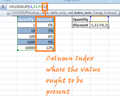
Step 5) Argument4: Last argument would be the condition for Approximate Matches or Exact Matches. In this instance, we are particularly looking for the Approximate matches (TRUE Keyword).

Step 6) Press ‘Enter.’ Vlookup formula will be applied to the mentioned Cell reference, and when you enter any number in the quantity field, it will show you the discount imposed based on Approximate Matches in VLOOKUP.

NOTE: If you want to use TRUE as the last parameter, you can leave it blank and by default it chooses TRUE for Approximate Matches.

VLOOKUP function applied between 2 different sheets placed in the same workbook

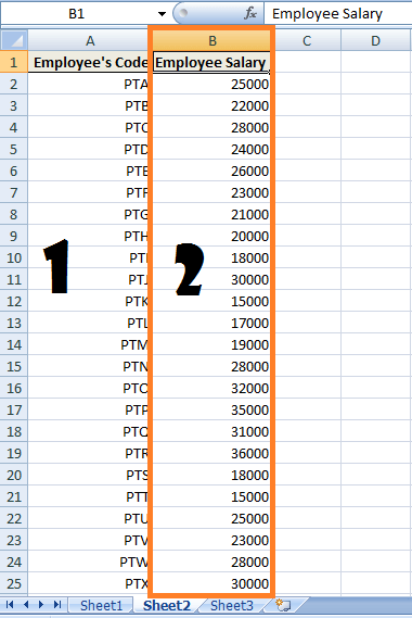
Let’s see an instance similar to the above case scenario. We are provided with one workbook containing two different sheets. One where Employee’s Code along with Employee’s Name and Employee’s Designation is given another sheet contains Employee’s Code and respective Employee’s Salary (as shown below).

SHEET 1:

SHEET 2:

Now the objective is to view all the data in one page, i.e., Sheet 1 as below:

VLOOKUP can help us aggregate all the data so that we can see Employee’s Code, Name, and Salary in one place or sheet.

We will start our work on Sheet 2 as that sheet provides us with two arguments of the VLOOKUP function that is – Employee’s Salary is listed in Sheet 2 which is to be searched by VLOOKUP and reference of the Column index is 2 (as per the lookup table).

Also, we know we want to find the employee’s salary corresponding to the Employee’s Code.

Moreover, that data starts in A2 and ends in B25. So that would be our lookup table or the table array argument.

Step 1) Navigate to sheet 1 and enter the respective headings as shown.

Step 2) Click on the cell where you want to apply the VLOOKUP function. In this case, it would be cell alongside Employee’s Salary with cell reference ‘F3’.

Enter the Vlookup function: =VLOOKUP ().

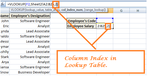
Step 3) Argument 1: Enter the cell reference which contains the value to be searched in the lookup table. In this case, ‘F2’ is the reference index which will contain Employee’s Code to match for corresponding Employee’s Salary in the lookup table.

Step 4) Argument 2: In the second argument, we enter the lookup table or the table array. However, in this instance, we have the lookup table situated in another sheet in the same workbook. Therefore, for building a relationship we need to enter address of the lookup table as Sheet2!A2:B25 – (A2:B25 refers to the lookup table in sheet 2)

Step 5) Argument 3: Third argument refers to the Column index of the column present in Lookup table where values ought to be present.

Step 6) Argument 4: Last Argument refers to the Exact Matches (FALSE) or Approximate Matches (TRUE). In this instance, we want to retrieve the exact matches for the Employee’s Salary.

Step 7) Press Enter and when you enter the Employee’s Code in the cell, you will be returned with corresponding Employee’s Salary for that Employee’s Code.

Conclusion

The above 3 scenarios explain the working of VLOOKUP Functions. You can play around using more instances. VLOOKUP is an important feature present in MS-Excel which allows you to manage data more efficiently.